BigData4Mobility
Open Source Dataset: GeoLife
Data Files and Variables
GeoLife trajectory file
| # | Column name | Type | Unit / format | Description |
|---|---|---|---|---|
| 1 | lat |
Float | Decimal (WGS-84) | Latitude |
| 2 | lon |
Float | Decimal (WGS-84) | Longitude |
| 3 | dummy |
Int | — (always 0) | Reserved placeholder |
| 4 | altitude_ft |
Float | Feet (–777 = missing) | Altitude above sea level |
| 5 | serial_days |
Float | Days since 1899-12-30 | Excel-style numeric datetime |
| 6 | date |
String | YYYY-MM-DD (GMT) | Calendar date (string form of #5) |
| 7 | time |
String | HH:MM:SS (GMT) | Time of day (string form of #5) |
Note: GeoLife data collected GPS trajectories by 182 users in a period from April 2007 to August 2012.
Transportation-mode label file (labels.txt)
| # | Column name | Type | Format | Description |
|---|---|---|---|---|
| 1 | start_time |
Datetime | YYYY/MM/DD HH:MM:SS (GMT) | Segment start |
| 2 | end_time |
Datetime | YYYY/MM/DD HH:MM:SS (GMT) | Segment end |
| 3 | mode |
String | walk, bike, bus, car … | User-annotated mode |
Note: 69 users have labeled their trajectories with transportation mode, such as driving, taking a bus, riding a bike or walking. The label files store the transportation mode labels for these users.
Data Characteristics
1. Data Stability
1.1 Number of devices per day over time
| Figure | Figure description |
|---|---|
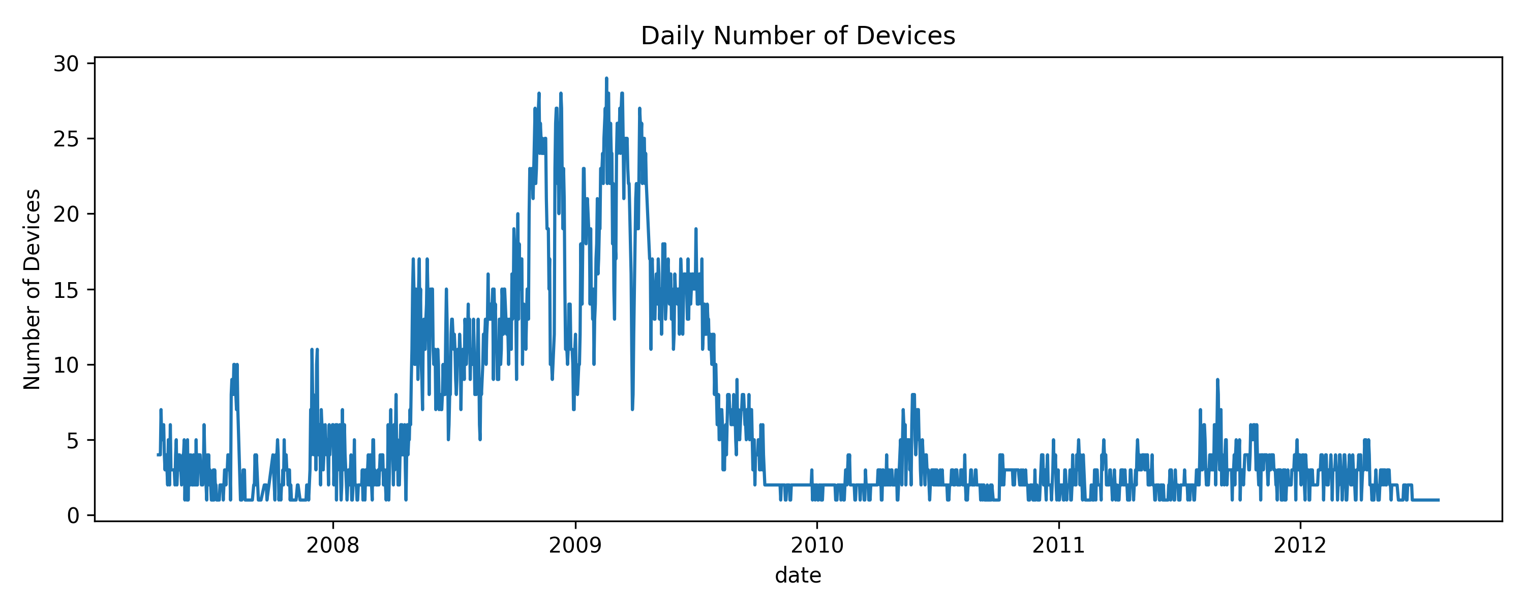 |
The horizontal axis is time (date), and the vertical axis is the number of devices with records on the corresponding date. |
Summary statistics of number of device per day for different years
| Statistic | All years | 2007 | 2008 | 2009 | 2010 | 2011 | 2012 |
|---|---|---|---|---|---|---|---|
| Mean | 5.93 | 3.32 | 10.54 | 11.70 | 2.43 | 2.74 | 2.21 |
| Standard deviation | 6.24 | 2.14 | 6.67 | 7.83 | 1.24 | 1.34 | 1.07 |
| Minimum | 1 | 1 | 1 | 1 | 1 | 1 | 1 |
| 25th percentile | 2 | 2 | 5 | 4 | 2 | 2 | 1 |
| Median | 3 | 3 | 10 | 12 | 2 | 3 | 2 |
| 75th percentile | 8 | 4 | 14 | 17 | 3 | 4 | 3 |
| Maximum | 29 | 11 | 28 | 29 | 8 | 9 | 5 |
Findings: From 2007 to 2012, the daily number of active devices (devices that have records on the corresponding date) ranges from 1 to 29, with an overall mean of 5.93, a median of 3, an inter-quartile range of 2 to 8, and a standard deviation of 6.24. The yearly averages fluctuate markedly: the mean is 3.32 devices in 2007, rises to 10.54 in 2008 and peaks at 11.70 in 2009, then falls to roughly 2–3 devices per day during 2010–2012, showing that this metric varies substantially over time rather than remaining stable.
1.2 Number of records per device per day over time
| Figure | Figure description |
|---|---|
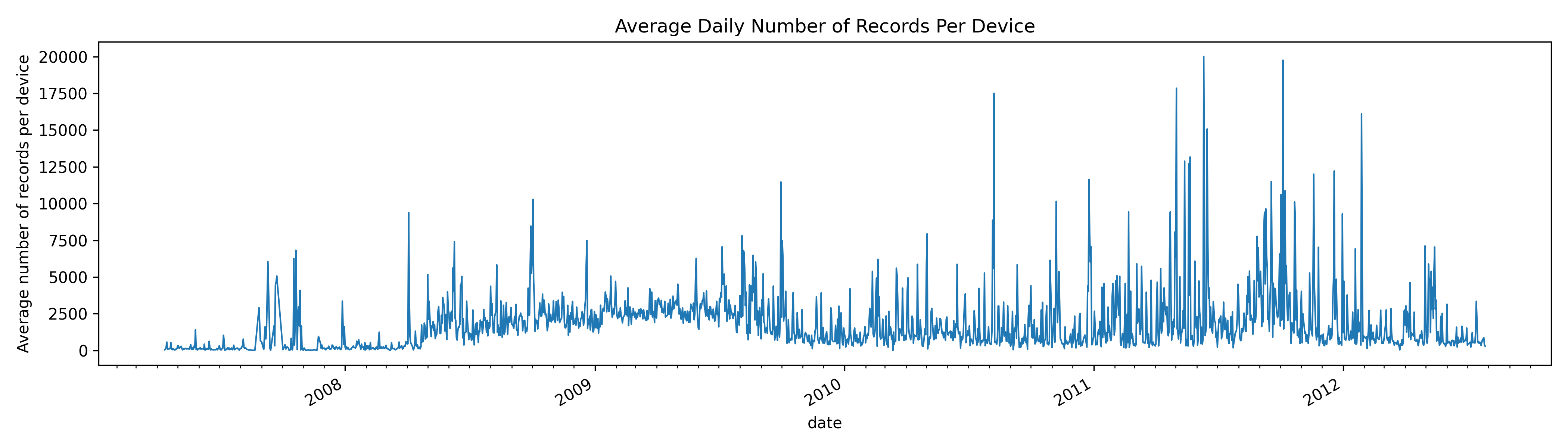 |
The horizontal axis is the time (date), and the vertical axis is the average daily number of records for devices with records on the corresponding date |
Summary statistics of number of records per device per day for different years
| Statistic | All years | 2007 | 2008 | 2009 | 2010 | 2011 | 2012 |
|---|---|---|---|---|---|---|---|
| mean | 2231.92 | 381.82 | 2126.66 | 2710.54 | 1620.70 | 2880.78 | 1490.19 |
| std | 3443.03 | 1488.90 | 3403.61 | 3274.69 | 2290.50 | 5298.79 | 2869.91 |
| min | 1.00 | 1.00 | 3.00 | 2.00 | 6.00 | 14.00 | 10.00 |
| 25th percentile | 457.00 | 37.00 | 432.50 | 742.25 | 501.00 | 551.00 | 440.50 |
| median | 1183.00 | 92.00 | 1184.50 | 1709.00 | 915.50 | 1254.50 | 692.00 |
| 75th percentile | 2788.00 | 214.00 | 2696.25 | 3525.25 | 1711.25 | 3085.00 | 1553.50 |
| max | 59769.00 | 20362.00 | 59769.00 | 50933.00 | 23799.00 | 56780.00 | 44808.00 |
Findings: From 2007 to 2012, the number of records per device per day changes a lot. On average a device logs about 2,232 records a day, but half the devices stay below 1,183 while at some day reaches 59,769. The mean is only 382 in 2007 (most days fall between 37 and 214 records). The average daily number of records per device climbs to 2,711 in 2009, drops to 1,620 in 2010, peaks at 2,881 in 2011, and then drops to 1,490 in 2012. The time-series plot shows the same story — many sharp spikes instead of a smooth curve — so the data jumps day to day and year to year rather than rising or falling steadily.
2. Temporal Sparsity
Temporal sparsity was investigated via two measures: intra-day temporal occupancy and inter-day temporal occupancy, quantifying how the device’s observations were distributed across different times within a day and across different days.
2.1 Intra-day Temporal Occupancy
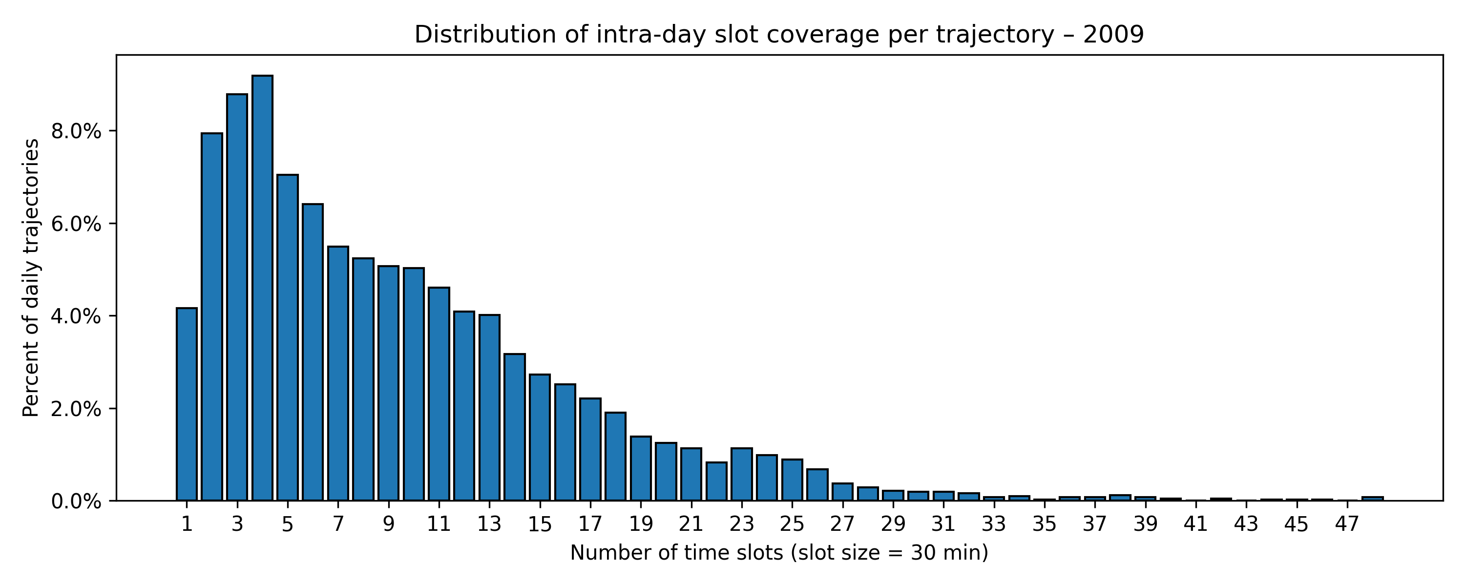
Description: Intra-day temporal occupancy measures the number of 30-minute time slots (total 48 slots) in a day in which a device was observed at least once (in the time slot). This measure is to capture the potential data sparsity within the day. For each trajectory (a sequence of records for a device in one day), we count how many 30-minute time slots the records of the trajectory cover and plot the percent of the number of trajectories with each number of 30-minute time slots to the total number of trajectories. We do calculations for each year and whole time period (all years).
| Figure | Figure |
|---|---|
 |
 |
 |
 |
 |
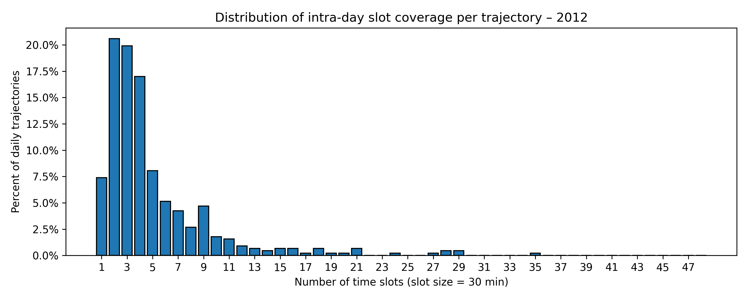 |
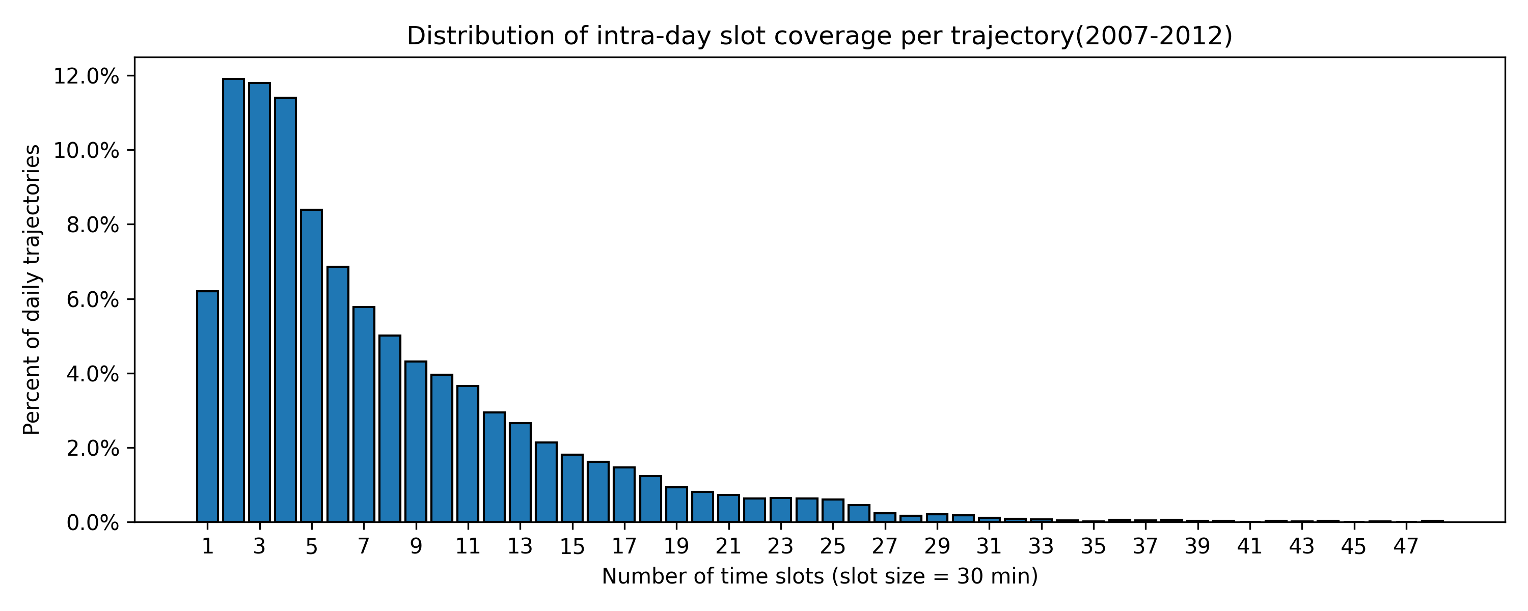
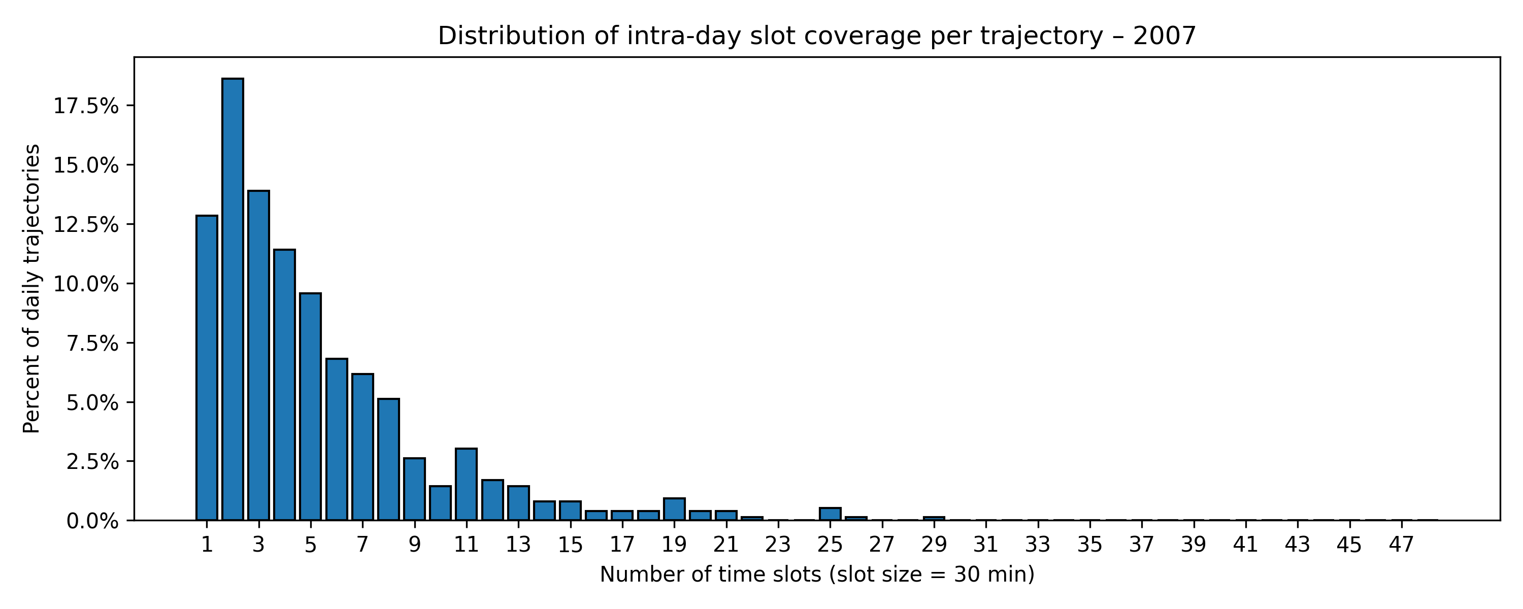
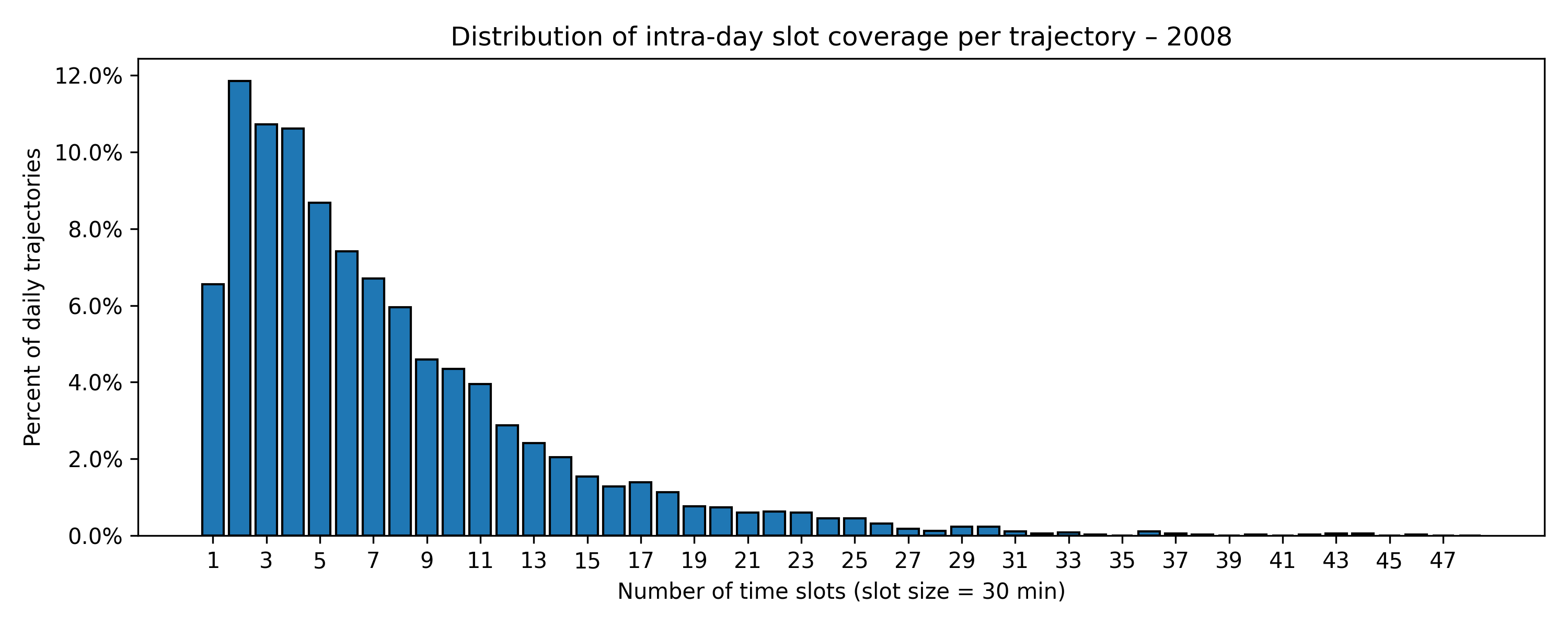
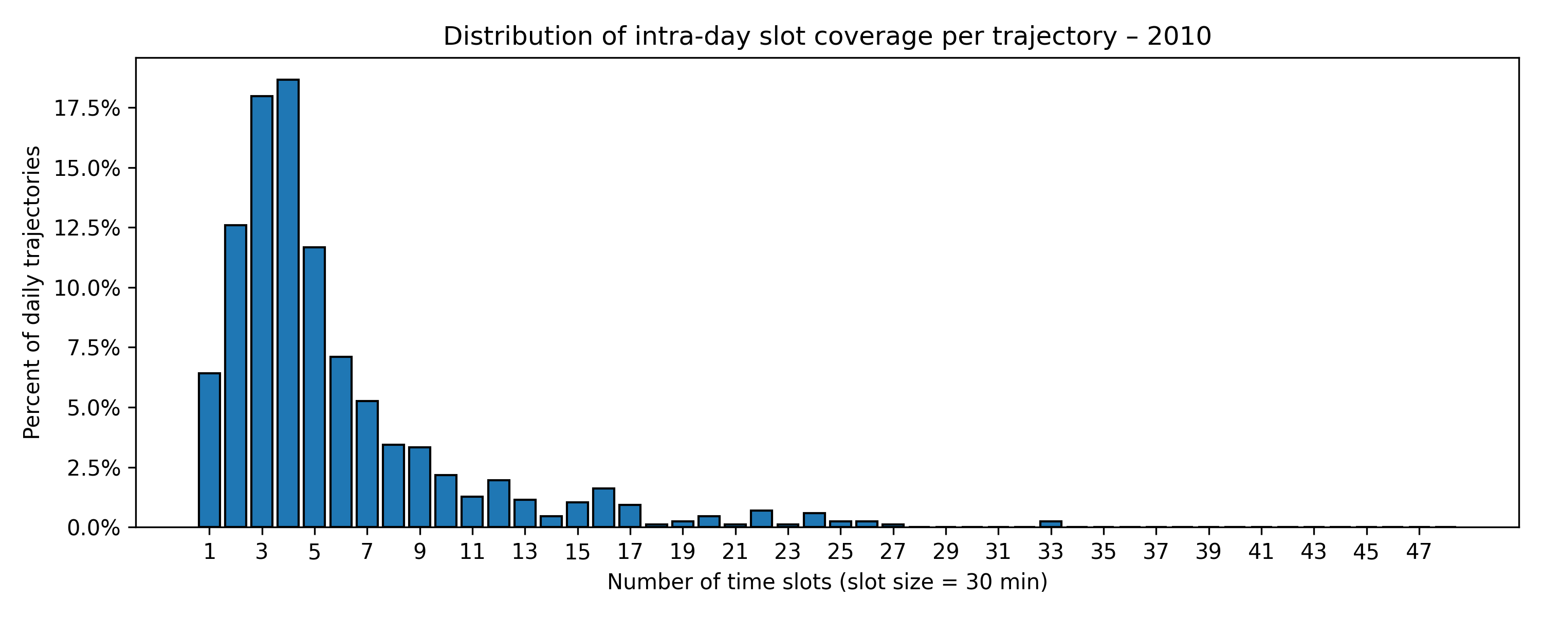
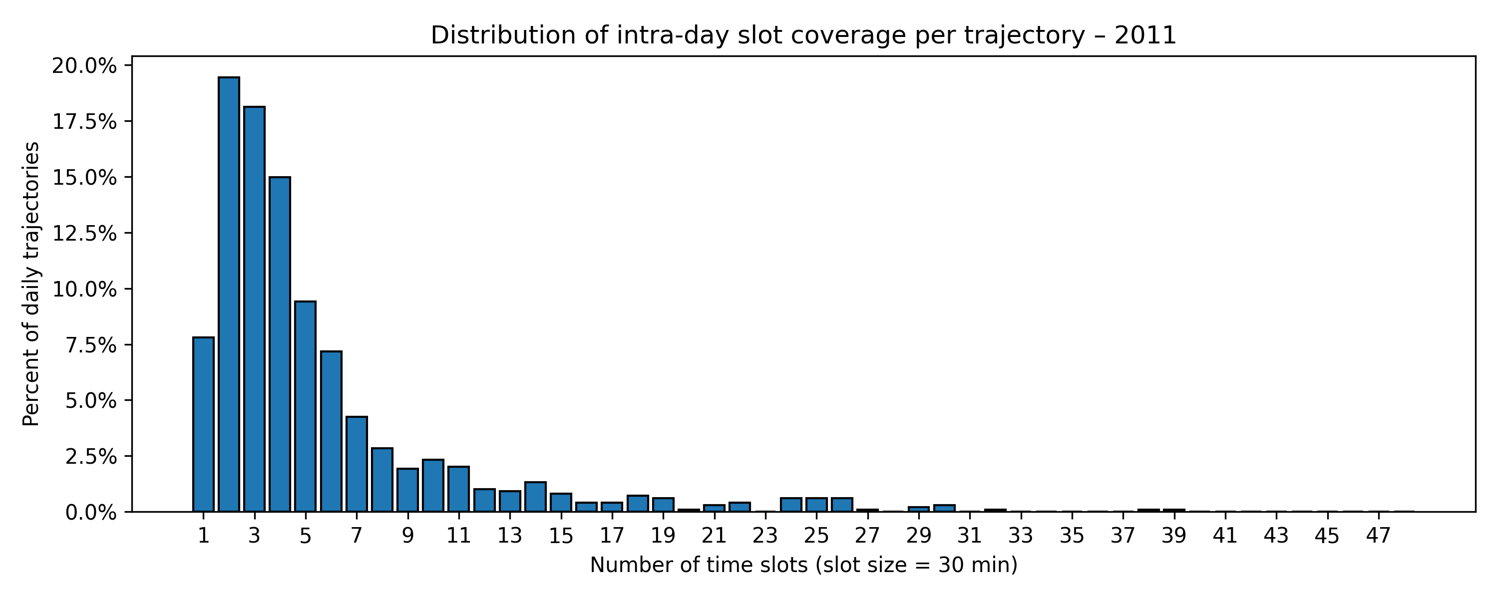
Figure Description: The horizontal axis is each number of 30-minute time slots in one day (there are 48 30-minute time slots in one day, ranging from 1 to 48), and the vertical axis is the percent of daily trajectories recorded in the corresponding number of time slots to the total trajectories. We plot the distribution of the intra-day occupancy for each year and whole time period (all years).
Summary statistics of Intra-day occupancy: number of time slots in one day a device was observed (slot size = 30 min, total 48 slots in one day)
| Statistic | All years | 2007 | 2008 | 2009 | 2010 | 2011 | 2012 |
|---|---|---|---|---|---|---|---|
| Mean | 7.60 | 5.20 | 7.43 | 9.35 | 5.64 | 5.50 | 5.06 |
| Standard deviation | 6.31 | 4.41 | 6.05 | 6.94 | 4.67 | 5.31 | 4.69 |
| Minimum | 1 | 1 | 1 | 1 | 1 | 1 | 1 |
| 25th percentile | 3 | 2 | 3 | 4 | 3 | 2 | 2 |
| Median | 6 | 4 | 6 | 8 | 4 | 4 | 4 |
| 75th percentile | 10 | 7 | 10 | 13 | 7 | 6 | 6 |
| Maximum | 48 | 29 | 46 | 48 | 33 | 39 | 35 |
Findings: Most daily traces are short. Across all years a device is seen in about 8 of the 48 half-hour slots per day on average—roughly 4 hours—but half of the traces last 3 hours or less, and one in four lasts only 1 ½ hours. The long tail is clear: only a small share of trajectories had their locations observed at each time slot (48 slots) in a day, yet most do not reach even half the day. Year-by-year, 2009 stands out with the longest coverage (mean 9.4 slots; median 8 slots), and 2008 is next (mean 7.4 slots; median 6 slots). By contrast, 2007, 2010, 2011, and 2012 all hover near 5–6 slots on average, with medians of just 4 slots (2 hours). These patterns indicate that the intensity of daily recordings differs across years.
2.2 Inter-day Temporal Occupancy
Description: Inter-day temporal occupancy measures the number of days within a time period (e.g., 6 months, one year, or the time period covered by the dataset) during which a device was observed at least once (in the day). This measure is to capture the data sparsity across different days within a time period. The GeoLife data was collected from April 2007 to August 2012 (total 1980 days), thus the inter-day occupancy we calculated for the whole study period (all years) are out of the total 1980 days, for 2007 and 2012 it is out of a partial year for 2007 (275 days) and 2012 (244 days), and for the other years (2008-2011), it is out of full one year.
| Figure | Figure |
|---|---|
Total number of days for 2007 (April - December): 275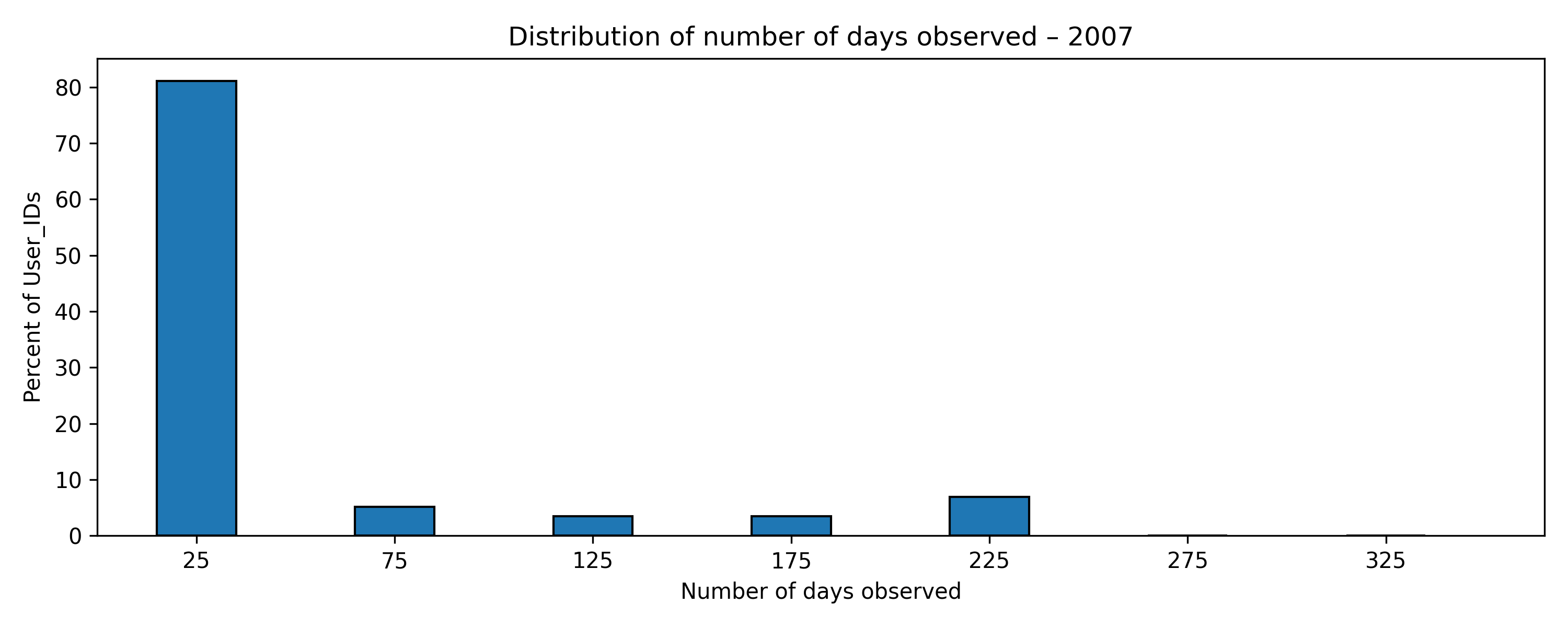 |
Total number of days for 2008: 366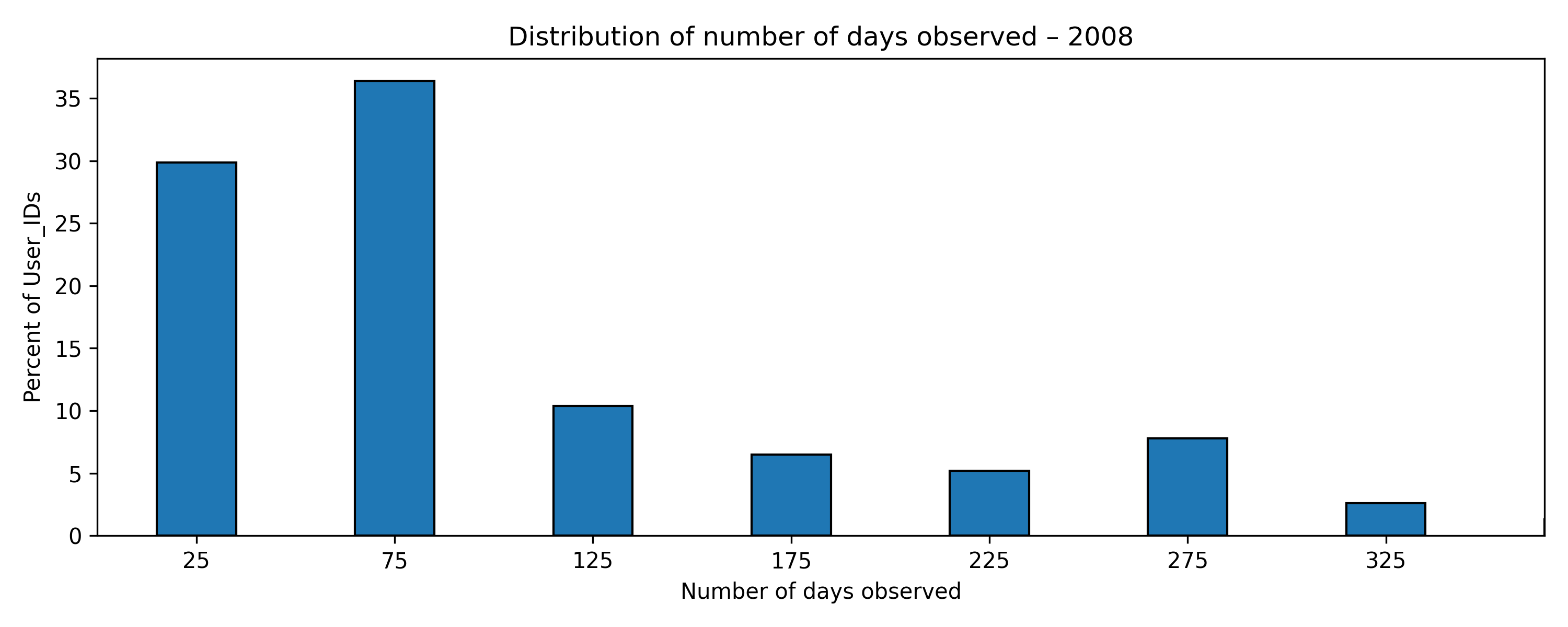 |
Total number of days for 2009: 365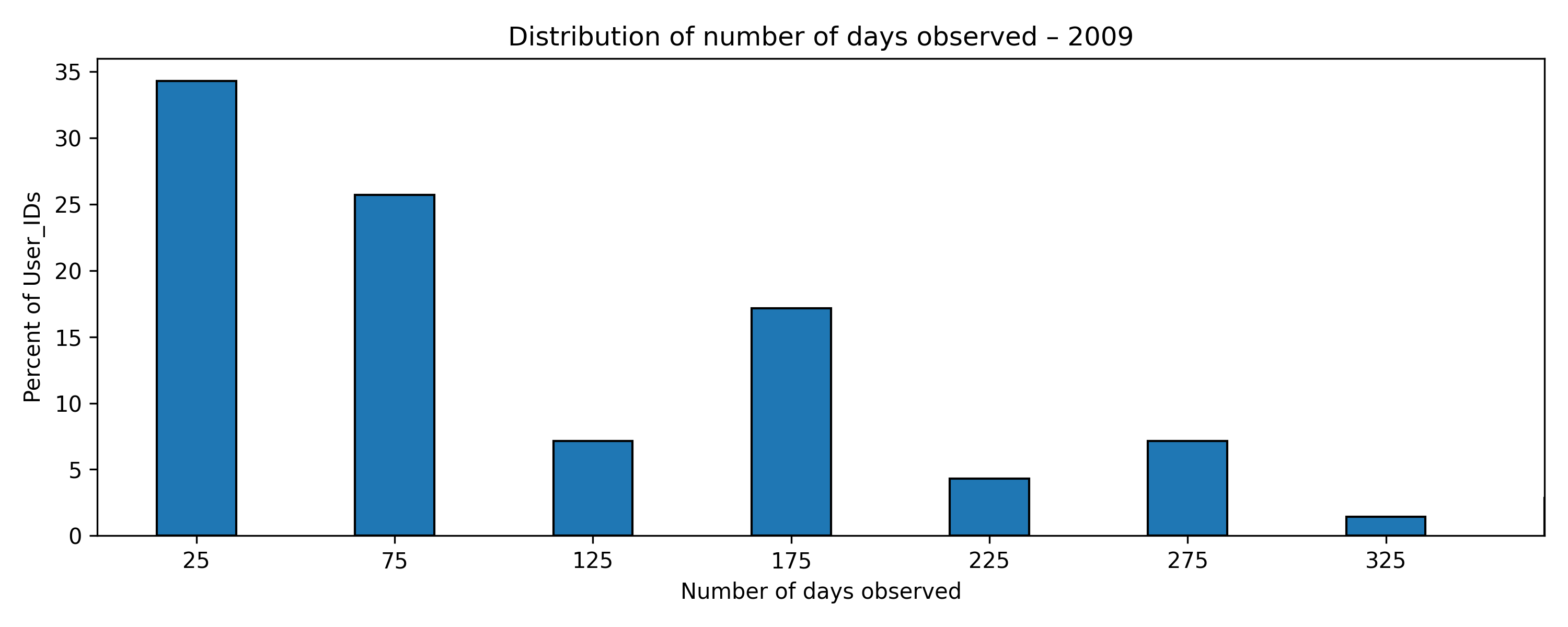 |
Total number of days for 2010: 365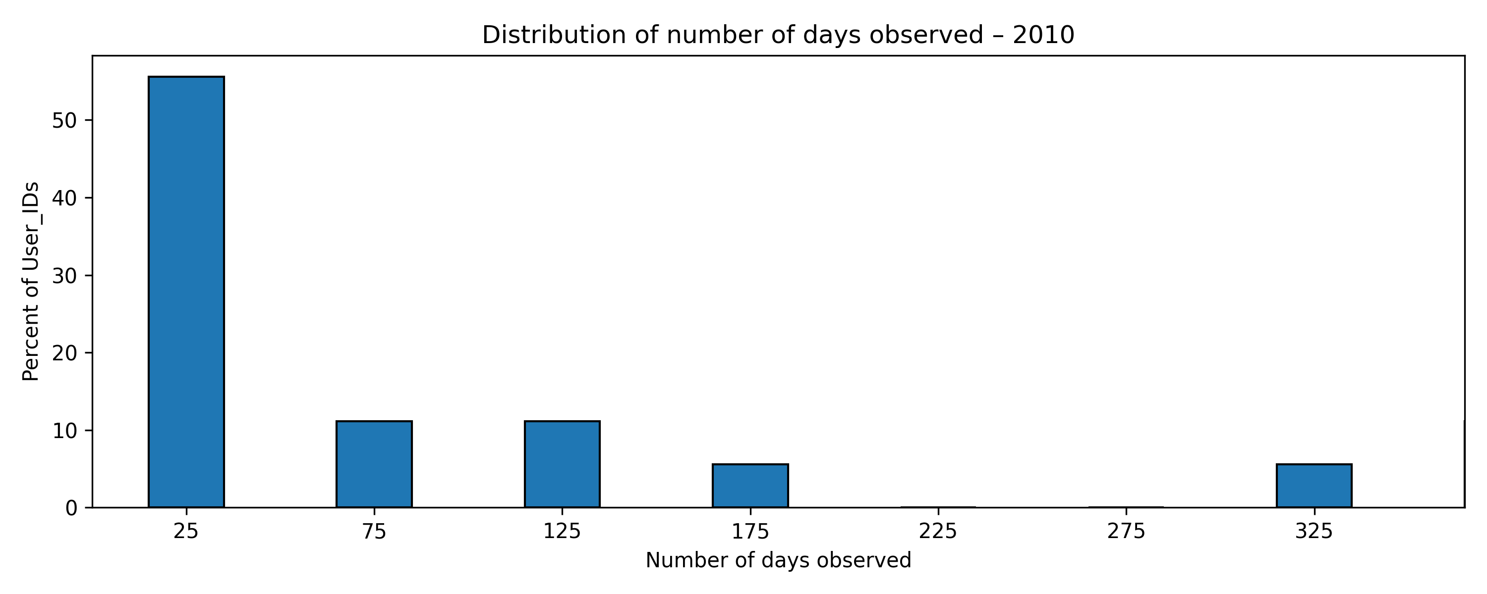 |
Total number of days for 2011: 365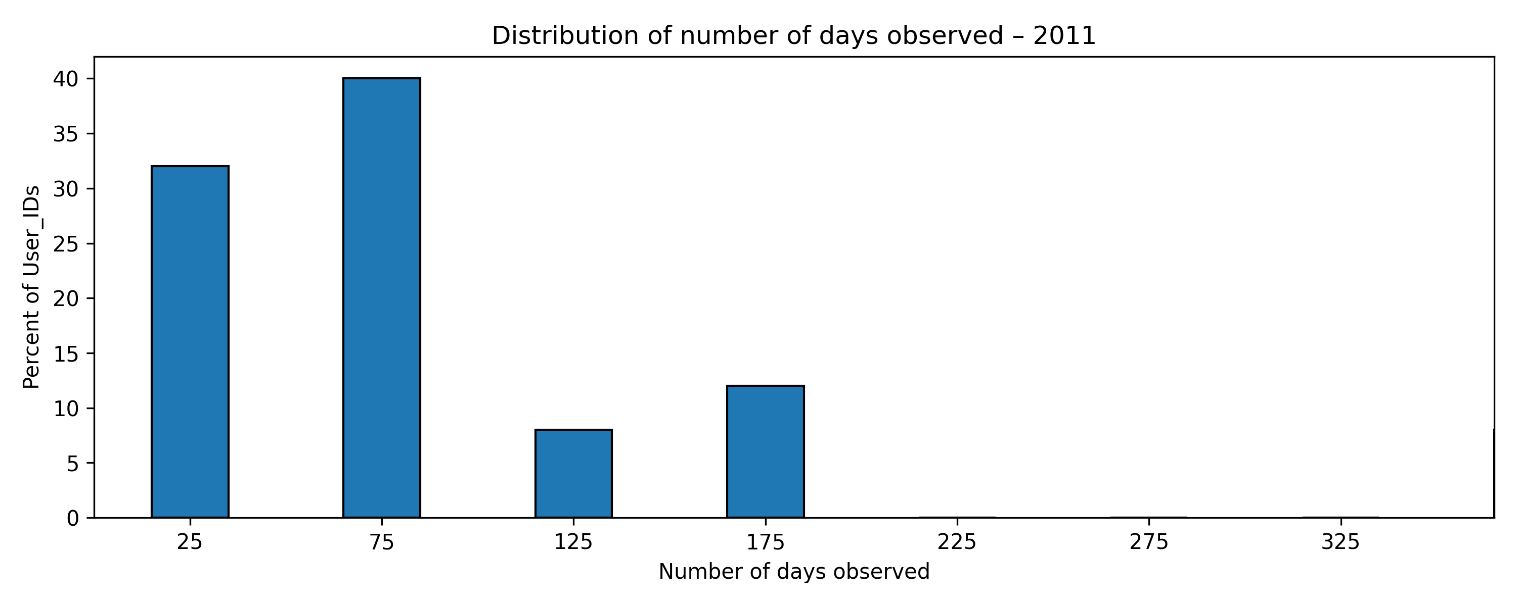 |
Total number of days for 2012 (January - August): 244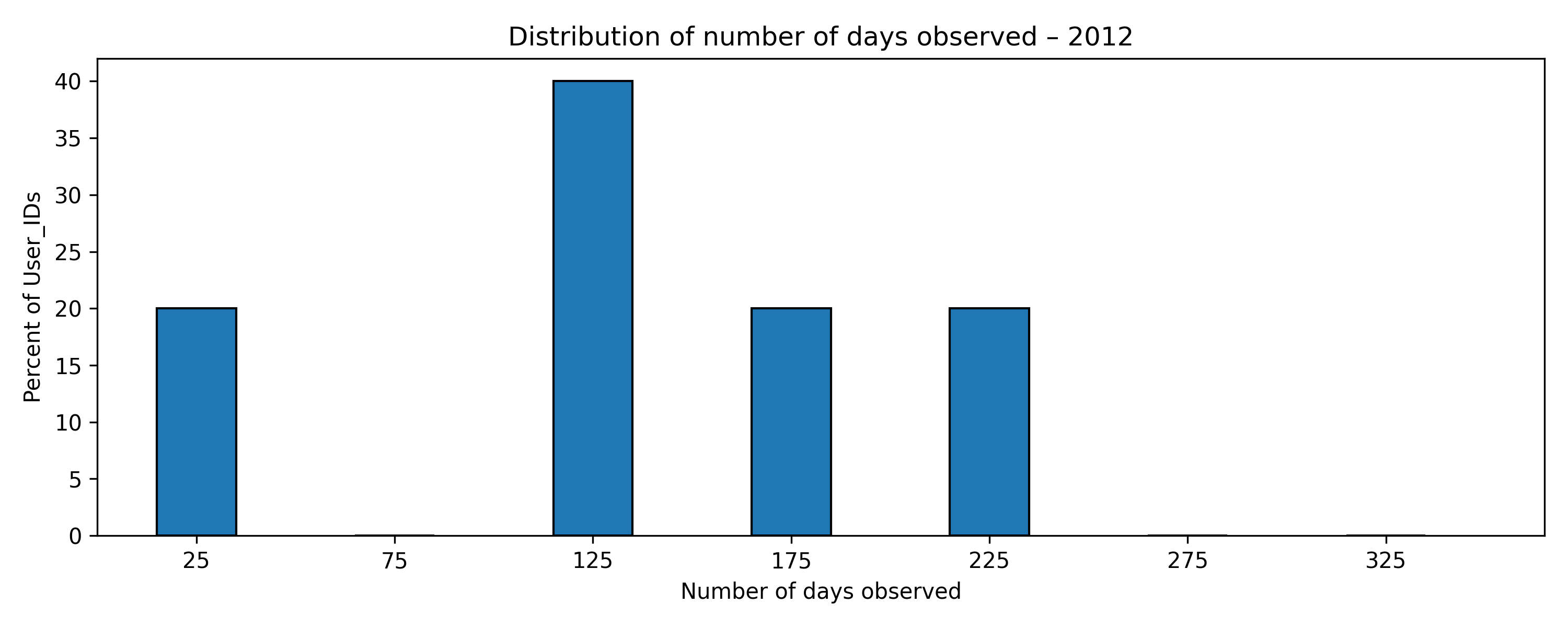 |
Total number of days for April 2007 - August 2012: 1980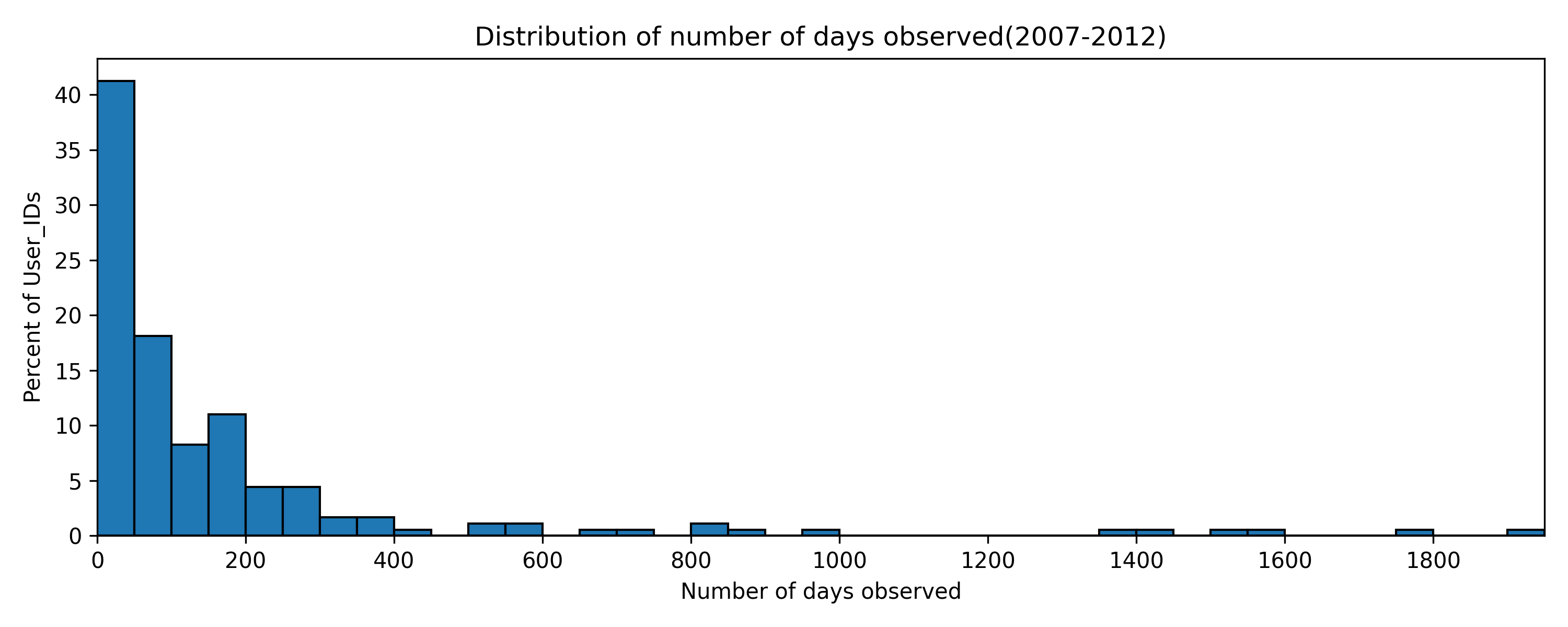
Figure Description: The horizontal axis is the number of days each device (user_id) was observed during a specific time period (e.g., one year), and the vertical axis is the percent of the number of device (user_ids) with the corresponding value in number of days observed to the total number of devices (user_ids).
Summary statistics of Inter-day occupancy: number of days a device was oberved during a specific time period
| Statistic | All years | 2007 | 2008 | 2009 | 2010 | 2011 | 2012 |
|---|---|---|---|---|---|---|---|
| Total number of days | 1980 | 275 | 366 | 365 | 365 | 365 | 244 |
| Mean | 174.41 | 41.57 | 99.88 | 106.29 | 98.22 | 92.00 | 134.80 |
| Standard deviation | 318.56 | 64.25 | 91.47 | 96.83 | 124.71 | 96.56 | 62.64 |
| Minimum | 1 | 1 | 1 | 1 | 1 | 1 | 41 |
| 25th percentile | 11 | 9 | 38 | 15 | 20.25 | 12 | 120 |
| Median | 71 | 12 | 70 | 83 | 29 | 68 | 135 |
| 75th percentile | 167.50 | 32 | 123 | 165 | 132.75 | 125 | 169 |
| Maximum | 1 934 | 242 | 350 | 365 | 365 | 365 | 209 |
Findings: Most devices are seen only part-time. Across the whole study window (1980 days), half of the devices appear on at most 71 days, and 75 % of them show up on fewer than 168 days (less than 10% of the total number of days in the study period). Only a small group is tracked for long stretches, but one very persistent device is present on 1934 days. Year-by-year patterns echo this limited reach: in 2007 (total 275 days in the study period) the average number of days a device was observed is just 42 days, while in 2008, 2010 and 2011 the mean hovers over 90 days out of 365 days. Two years stand out: in 2009 a typical device is recorded on 106 of the 365 days (about 29 % of the year); and in 2012—when data run only from 1 January to 31 August (244 days)—the mean rises to 135 days, or roughly 55 % of the study period.
3. Temporal Gap
Description: Temporal gap refers to the time interval between consecutive location observations for a single device in LBS data. It is another indicator of data continuity. A small temporal gap implies high-frequency location sampling, while large temporal gaps suggest that significant portions of a user’s movement may go unobserved.
| Figure | Figure discription |
|---|---|
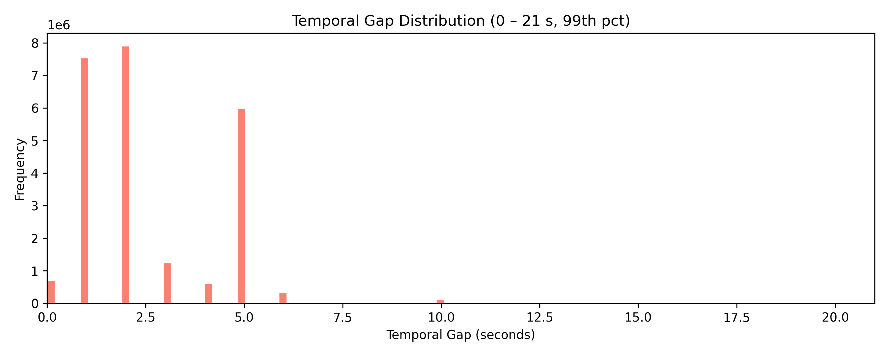 |
The horizontal axis represents the temporal gap value (time interval in seconds) for a device, and the vertical axis represents the number of records corresponding to the temporal gap value. (The upper bound of the horizontal axis is set at the 99th percentile of the gap distribution.) |
Summary statistics of temporal gaps (seconds)
| Statistic | Value (seconds) |
|---|---|
| Mean | 109.61 |
| Standard deviation | 46,652.38 |
| Minimum | 0 |
| 25th percentile | 1 |
| Median | 2 |
| 75th percentile | 5 |
| 95th percentile | 5 |
| 99th percentile | 21 |
| Maximum | 1,257,394 |
Findings: Most pairs of points are recorded very close in time: 50 % are within 2 seconds, 95 % within 5 seconds, and 99 % within 21 seconds, indicating that the majority of observations occur within short intervals in GeoLife data. Only a few very long gaps — up to about 1.26 million seconds (nearly 4 years) — pull the average up to 110 seconds and give a wide spread, so the distribution is strongly right-skewed.
4. Spatial Gap
Description: Spatial gap (also termed “jumping distance”) refers to the distance between consecutive location observations for a single device in LBS data. It is a critical metric for assessing the continuity and reliability of reconstructed travel trajectories. A small spatial gap suggests frequent location updates, while large spatial gaps indicate that a user’s location was not observed for an extended portion of their movement, potentially missing entire trips or key trajectory segments.
| Figure | Figure description |
|---|---|
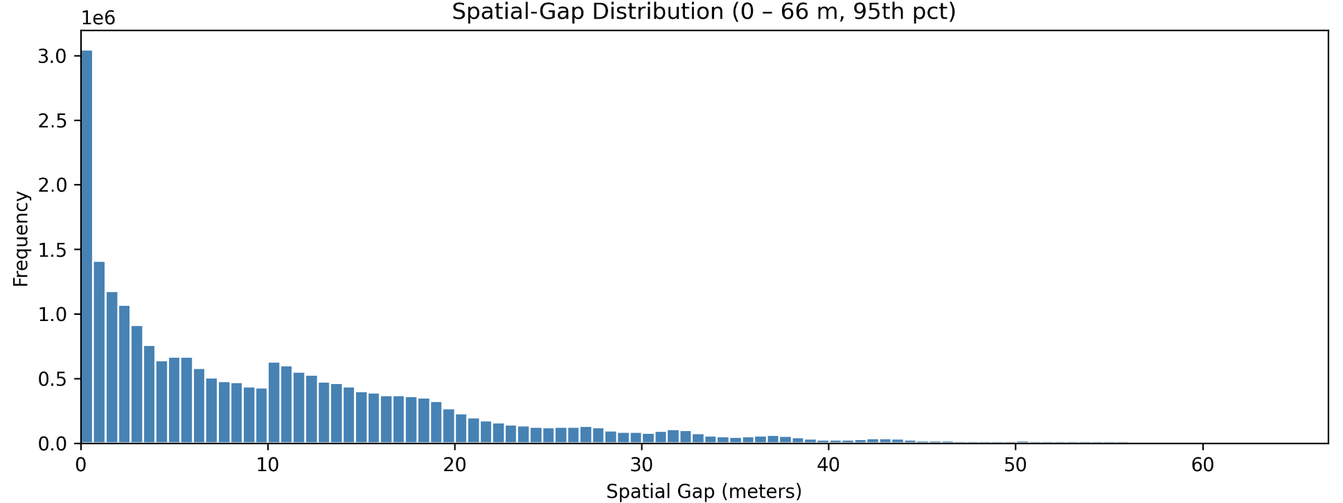 |
The horizontal axis represents the distance (in meters) between two adjacent records for a device, and the vertical axis represents the number of records with the corresponding distance. (The upper bound of the horizontal axis is set at the 95th percentile of the gap distribution.) |
Summary statistics of spatial gaps (meters)
| Statistic | Value (meters) |
|---|---|
| Mean | 73.24 |
| Standard deviation | 11,919.00 |
| Minimum | 0 |
| 25th percentile | 2.36 |
| Median | 8.73 |
| 75th percentile | 17.64 |
| 95th percentile | 66.70 |
| 99th percentile | 190.95 |
| Maximum | 11,129,650 |
Findings: The spatial gap distribution is strongly right-skewed: the mean distance between consecutive location observations for device is about 73 m, yet the standard deviation exceeds 11 km. The 25th, 50th, and 75th percentiles are roughly 2.4 m, 8.7 m, and 17.6 m, respectively, indicating that three-quarters of gaps are below 18 m. The minimum gap is 0 m, whereas the maximum exceeds 11 000 km, revealing the presence of a small number of extreme long-distance intervals within the data.
5. Precision
The spatial accuracy (uncertainty radius) information is not provided in the GeoLife data, so the spatial precision of the GeoLife data is unknown.
6. Representation
The information about how the 182 users were selected in the GeoLife data has not been found. This group is compared to a larger population of 19,612,368 in Beijing, China, based on the 2010 6th China Census (Source: Data from National Bureau of Statistics of China).
The lack of details on how these 182 users were selected introduces potential representation bias. Without information on the selection criteria, it is unclear whether this sample accurately reflects the broader Beijing population, which may have varied demographics and behaviors. If the sample was not randomly chosen, it could overrepresent certain groups (e.g., tech-savvy individuals) or underrepresent others (e.g., people with limited access to technology), affecting the generalizability of the data to the entire population.